Research Question
Which variables show the highest likelihood of customers leaving the company, based on three explanatory variables from the churn database. The ‘churn’ variable is the target variable.
Goal
Using known variables within a dataset, analysts can predict which customers are more likely to leave in the future by using KNN classification. This is helpful for decision makers to know how to adjust certain services offered and which variables are at risk to leaving, to keep customers longer.
Method Justification: Classification Method
For KNN classification algorithm for this task, is a method of classifying data points based on the distance of the closest neighbors. This is particularly useful when training the dataset for look-alike data points. Once a dataset is trained any new data points that come in can be classified based on the nearest neighbors. Expected outcomes will be using the training dataset to run accuracy of the testing data points in the Churn dataset. Based on three variables: income, tenure, and bandwidth usage this knn model will classify new customers on whether they will leave the company or not. (Sree, 2020)
Method Assumption:
In this task, KNN method assumes that within a certain set distance, that data points are similar. (Grant, 2019)
Packages and Libraries:
The Python packages and libraries used in this task are:
- Scikit-learn: predictive and classification analysis is ran in this package for this task. To find the AUC score this packages was used too.
- Matplotlib: one of the most common graph plots Matplotlib package, is used in this task.
- Numpy: was used to compute the array operations for this task. (Koidan, 2021)
Python is the programming language used to run stats, analysis, models, and research for this task. Python comes with several packages that will be used for various parts of this analysis. Python makes it easy to run classification models and statistics on large datasets like the churn dataset. Jupyter Notebook is an online kernel to run Python using a web browser to import more packages, and libraries. Anaconda Navigator application runs Jupyter Notebook within a web browser and command prompt local sever. Anaconda Navigator has more than one thousand data sciences packages built in, which is easy to install and run. A MacBook pro laptop is used to install Anaconda application, run Python, export, and save datasets as well as save Jupyter Notebooks of Python code for future use.
Data Preparation: Data Preprocessing
Several of the variables are binary (yes/no), in order to use these they must be changed to numeric as dummy variables (0/1).
Dataset Variables
The ‘churn’ dataset has 50 variables ranging from information about the customer to details around individual subscription services. For this KNN model three variables remain that are relevant to the research question.
The dropped variables are: ‘Population’, ‘Children’, ‘Age’, ‘Outage_sec_perweek’, ‘Multiple’, ‘StreamingTV’, ‘StreamingMovies’, ‘CaseOrder’, ‘Customer_id’, ‘Interaction’, ‘UID’, ‘City’, ‘State’, ‘County’, ‘Zip’, ‘Lat’, ‘Lng’, ‘Area’, ‘MonthlyCharge’, ‘TimeZone’, ‘Job’, ‘Marital’, ‘Gender’, ‘Churn’, ‘Email’, ‘Contacts’, ‘Yearly_equip_failure’, ‘Techie’, ‘Contract’, ‘Port_modem’, ‘Tablet’, ‘InternetService’, ‘Phone’, ‘OnlineSecurity’, ‘OnlineBackup’, ‘DeviceProtection’, ‘TechSupport’, ‘PaperlessBilling’, ‘PaymentMethod’, ‘Item1’, ‘Item2’, ‘Item3’, ‘Item4’, ‘Item5’, ‘Item6’, ‘Item7’, ‘Item8’.
The variables that remain are numerical independent, including the target variable (churn): ‘Income’, ‘Tenure’, and ‘Bandwidth_GB_Year’. The mean income is 39806.926771 (with std: 28199.916702). The mean tenure months is 34.5 (std: 26.443063). And the mean bandwidth used per year is 3392.34GB/Year (std: 2185.294852).
Re-encode ‘churn’ binary (yes/no) categorical to numbers; by replacing “No” answers to “0’s” and “Yes” answers with “1’s”.
Steps for Analysis
- Import Python libraries
- Select: Import churn dataset into Python and determine which variables best answer the research question.
- Find and treat nulls: Look for missing data and treat those.
- Remove unrelated variables: Using the .drop() function, remove variables that aren’t correlated to the research question.
- Find and treat outliers: Look for outliers within the remaining variables and remove those using percentile’s function.
- Convert categorical data: To use categorical variables in the KNN model, these need to be converted from categorical to numeric
- Extract cleaned dataset as “dataset.csv” for use in KNN model
# Standard data science imports
import numpy as np

import pandas as pd
from pandas import Series, DataFrame

# Visualization libraries
import seaborn as sns

import matplotlib.pyplot as plt
%matplotlib inline

# Statistics packages
import pylab
from pylab import rcParams
import statsmodels.api as sm
import statistics
from scipy import stats

# Scikit-learn
import sklearn
from sklearn import preprocessing
from sklearn.linear_model import LinearRegression
from sklearn.model_selection import train_test_split
from sklearn import metrics
from sklearn.metrics import classification_report

# Import chisquare from SciPy.stats
from scipy.stats import chisquare
from scipy.stats import chi2_contingency

from sklearn.datasets import make_classification

from matplotlib import pyplot as plt
from sklearn.linear_model import LogisticRegression
from sklearn.model_selection import train_test_split
from sklearn.metrics import confusion_matrix
import pandas as pd
import statsmodels.api as sm

# Load data set into Pandas dataframe
dataset = pd.read_csv('/Users/rednebula/Desktop/churn_clean.csv')

dataset.info()

<class 'pandas.core.frame.DataFrame'>
RangeIndex: 10000 entries, 0 to 9999
Data columns (total 50 columns):
 #   Column                Non-Null Count  Dtype
---  ------                --------------  -----
 0   CaseOrder             10000 non-null  int64
 1   Customer_id           10000 non-null  object
 2   Interaction           10000 non-null  object
 3   UID                   10000 non-null  object
 4   City                  10000 non-null  object
 5   State                 10000 non-null  object
 6   County                10000 non-null  object
 7   Zip                   10000 non-null  int64
 8   Lat                   10000 non-null  float64
 9   Lng                   10000 non-null  float64
 10  Population            10000 non-null  int64
 11  Area                  10000 non-null  object
 12  TimeZone              10000 non-null  object
 13  Job                   10000 non-null  object
 14  Children              10000 non-null  int64
 15  Age                   10000 non-null  int64
 16  Income                10000 non-null  float64
 17  Marital               10000 non-null  object
 18  Gender                10000 non-null  object
 19  Churn                 10000 non-null  object
 20  Outage_sec_perweek    10000 non-null  float64
 21  Email                 10000 non-null  int64
 22  Contacts              10000 non-null  int64
 23  Yearly_equip_failure  10000 non-null  int64
 24  Techie                10000 non-null  object
 25  Contract              10000 non-null  object
 26  Port_modem            10000 non-null  object
 27  Tablet                10000 non-null  object
 28  InternetService       10000 non-null  object
 29  Phone                 10000 non-null  object
 30  Multiple              10000 non-null  object
 31  OnlineSecurity        10000 non-null  object
 32  OnlineBackup          10000 non-null  object
 33  DeviceProtection      10000 non-null  object
 34  TechSupport           10000 non-null  object
 35  StreamingTV           10000 non-null  object
 36  StreamingMovies       10000 non-null  object
 37  PaperlessBilling      10000 non-null  object
 38  PaymentMethod         10000 non-null  object
 39  Tenure                10000 non-null  float64
 40  MonthlyCharge         10000 non-null  float64
 41  Bandwidth_GB_Year     10000 non-null  float64
 42  Item1                 10000 non-null  int64
 43  Item2                 10000 non-null  int64
 44  Item3                 10000 non-null  int64
 45  Item4                 10000 non-null  int64
 46  Item5                 10000 non-null  int64
 47  Item6                 10000 non-null  int64
 48  Item7                 10000 non-null  int64
 49  Item8                 10000 non-null  int64
dtypes: float64(7), int64(16), object(27)
memory usage: 3.8+ MB

print(dataset['Churn'].value_counts())
sns.countplot(x='Churn', data=dataset, palette='hls')
plt.show()
No     7350
Yes    2650
Name: Churn, dtype: int64

# will replace "Yes" value in dataframe with 1
dataset['churn_dummy'] = [1 if v == 'Yes' else 0 for v in dataset['Churn']]

dataset.groupby('Churn').mean().round(2).T
| Churn | No | Yes |
| CaseOrder | 5710.00 | 3032.65 |
| Zip | 49017.78 | 49529.24 |
| Lat | 38.73 | 38.84 |
| Lng | -90.74 | -90.90 |
| Population | 9830.51 | 9551.46 |
| Children | 2.09 | 2.07 |
| Age | 53.01 | 53.27 |
| Income | 39706.40 | 40085.76 |
| Outage_sec_perweek | 10.00 | 10.00 |
| 11.99 | 12.08 | |
| Contacts | 0.99 | 1.01 |
| Yearly_equip_failure | 0.40 | 0.38 |
| Tenure | 42.23 | 13.15 |
| MonthlyCharge | 163.01 | 199.30 |
| Bandwidth_GB_Year | 3971.86 | 1785.01 |
| Item1 | 3.50 | 3.48 |
| Item2 | 3.51 | 3.48 |
| Item3 | 3.49 | 3.47 |
| Item4 | 3.50 | 3.49 |
| Item5 | 3.50 | 3.47 |
| Item6 | 3.50 | 3.50 |
| Item7 | 3.51 | 3.49 |
| Item8 | 3.49 | 3.51 |
| churn_dummy | 0.00 | 1.00 |
dataset.to_csv(r'/Users/rednebula/Desktop/dataset.csv')

knn_df = dataset[['Income', 'Tenure', 'Bandwidth_GB_Year', 'churn_dummy']]

knn_df.describe()
| Income | Tenure | Bandwidth_GB_Year | churn_dummy | |
| count | 10000.000000 | 10000.000000 | 10000.000000 | 10000.000000 |
| mean | 39806.926771 | 34.526188 | 3392.341550 | 0.265000 |
| std | 28199.916702 | 26.443063 | 2185.294852 | 0.441355 |
| min | 348.670000 | 1.000259 | 155.506715 | 0.000000 |
| 25% | 19224.717500 | 7.917694 | 1236.470827 | 0.000000 |
| 50% | 33170.605000 | 35.430507 | 3279.536903 | 0.000000 |
| 75% | 53246.170000 | 61.479795 | 5586.141370 | 1.000000 |
| max | 258900.700000 | 71.999280 | 7158.981530 | 1.000000 |
‘dataset.csv.’ dataset attached
- Analysis – knn
- Re-encode churn to numbers
- Save churn variable + 3 independent variables to knn dataframe
- Train dataset – fit
- K = 6
- Output for churn
- Accuracy score for churn
- Find best k number
- Auc score
Part 4: Analysis
D1. Splitting the Data
Using Python with Scikit-learn package add-on, the churn dataset was split into 80% train and 20% test data. Estimating, out of 10,000 customers, there were 2,000 in the test set out, and 8,000 were the training set model. Below is the code for achieving this as well as the KNN score of 77%. from sklearn.neighbors import KNeighborsClassifier
from sklearn.model_selection import train_test_split

X = knn_df.iloc[:, 1:-1].values
y = knn_df.iloc[:, -1].values

X_train, X_test, y_train, y_test = train_test_split(
            X, y, test_size = 0.2, random_state=42)

knn = KNeighborsClassifier(n_neighbors=6)

knn.fit(X_train, y_train)

print(knn.predict(X_test))
[0 1 1 ... 0 0 0]

In [14]:
print(knn.score(X_test, y_test))

0.768
Calculations
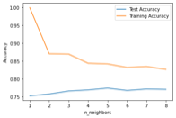
Using Python with Scikit-learn package add-on, the churn dataset was split into 80% train and 20% test data. Below is the code and plot of fitting the data into the model, using KNN (K Nearest Neighbor) classification algorithm, with an output of values vs accuracy. (w3resource)
import numpy as np
import matplotlib.pyplot as plt

X_train, X_test, y_train, y_test = train_test_split(
            X, y, test_size = 0.2, random_state=42)

neighbors = np.arange(1, 9)
train_accuracy = np.empty(len(neighbors))
test_accuracy = np.empty(len(neighbors))

for i, k in enumerate(neighbors):
    knn = KNeighborsClassifier(n_neighbors=k)
    knn.fit(X_train, y_train)
    train_accuracy[i] = knn.score(X_train, y_train)
    test_accuracy[i] = knn.score(X_test, y_test)

plt.plot(neighbors, test_accuracy, label = 'Test Accuracy')
plt.plot(neighbors, train_accuracy, label = 'Training Accuracy')

plt.legend()
plt.xlabel('n_neighbors')
plt.ylabel('Accuracy')
plt.show()
Code
from sklearn.metrics
import roc_curvepred_prob = knn.predict_proba(X_test)

fpr2, tpr2, thresh2 = roc_curve(y_test, pred_prob[:,1], pos_label=1)

random_probs = [0 for i in range(len(y_test))]
p_fpr, p_tpr, _ = roc_curve(y_test, random_probs, pos_label=1)
from sklearn.metrics import roc_auc_score

auc_score = roc_auc_score(y_test, pred_prob[:,1])

print(auc_score)
0.8297858506383322
Data Summary and Implications
Accuracy & AUC
The best score for this KNN model is k = 6. The accuracy model shows the training dataset drops in half in the first 2 k neighbors. Meaning k = 5, 6, 7, 8 is better for the algorithm. The accuracy score shows 77% – 79%; where the AUC (Area Under Curve) score is 83%.
Results & Implications
This supervised machine learning algorithm model shows, based on variables (Income, Tenure, and Bandwidth per year), it can accurately classify whether someone will churn or not 83% of the time.
Limitation
Using the KNN classification method, picking different numbers for k to train the model will yield different results. This is the bedrock of this classification model and algorithm. Because of this, each analysis can be much different based on the use of this number for “k”. It’s up to the analyst which number they want to use to train their model. We need more variables to accurately train this model.
Action
It’s important for this companies’ decision makers to know that this is a classification method, a way to predict certain services will be at a greater risk for their customers to leave. For this example, finding patterns between the longevity of their customers, how much money they make and how much bandwidth they consume can steer marketers into grouping new customers coming in. Offering a discount or free month of service for these customers who have been there a long time and are all about saving money might go a long way in retaining customers.
Sources for Third-Party Code
Sree. (2020, October 26). Predict Customer Churn in Python. Towards Data Science. https://towardsdatascience.com/predict-customer-churn-in-python-e8cd6d3aaa7
(2022, August 19). Python Scikit-learn: K Nearest Neighbors – Create a plot of k values vs accuracy. W3resource. https://www.w3resource.com/machine-learning/scikit-learn/iris/python-machine-learning-k-nearest-neighbors-algorithm-exercise-8.php
Sources Grant, P. (2019, July 21). Introducing k-Nearest Neighbors. TowardDataScience. https://towardsdatascience.com/introducing-k-nearest-neighbors-7bcd10f938c5
(2022, August 19). Python Scikit-learn: K Nearest Neighbors – Create a plot of k values vs accuracy. W3resource. https://www.w3resource.com/machine-learning/scikit-learn/iris/python-machine-learning-k-nearest-neighbors-algorithm-exercise-8
Koidan, Kateryna. (2021, August 19). Most Popular Python Packages in 2021. LearnPython https://learnpython.com/blog/most-popular-python-packages/