IMDb Rating ML Regression Model

Research Question

What is the anticipated IMDb (Internet Movie Database) rating a movie can achieve by leveraging a set of explanatory variables extracted from a popular movie database?

IMDb.com is the largest internet movie database, featuring popular user ratings, reviews for movies and shows, and more. Ranked as the 52nd most visited website in 2019, this site began as a fan-operated movie database and has been owned and operated by Amazon since 1998. The rating variable in this dataset serves as an indicator of a movie’s popularity among both fans and critics. Identifying the variables that exhibit strong correlations with higher ratings can enhance predictive modeling for the cinema industry.

The established null and alternative hypotheses for this analysis project is:

Null hypothesis – The independent variables have no effect on the dependent variable, average IMDb movie rating of “high” or “low” from the Internet Movie Database.

Alternate hypothesis – The independent variables influence the dependent variable, average IMDb movie rating of “high” or “low” from the Internet Movie Database.

To successfully build a logistic regression model for predicting a movie’s rating based on independent variables, the null hypothesis must be rejected, and the alternate hypothesis must be validated as accurate. If an effective model is generated, it can then be used to predict the rating of a new movie.

Data Collection

The dataset downloaded from Kaggle called, “IMDB Top 10,000 movies” consisted of the following variables:

title: The name/title of the movie.
year: The release year of the movie.
runtime: The total duration/length of the movie in minutes.
certificate: The age certification or rating of the movie (e.g., PG, R, U/A).
genre: The category or type of movie (e.g., Drama, Action, Romance).
director: The director of the movie.
stars: Leading actors and actresses featured in the movie.
rating: The average IMDB rating of the movie out of 10.
metascore: The metascore rating based on critical reviews.
votes: The total number of user votes/ratings the movie received on IMDB.
gross: The total box office collection/gross earnings of the movie in millions.

This dataset, updated in August 2023, consists of public data web-scraped from IMDb.com from a python script into a .csv file for download. This dataset showcases a comprehensive list of IMDB’s top-rated movies. It offers an extensive glimpse into the insights that define a film’s success and its place in cinematic history. The rating variable is the target variable used for predication from the set of cinema numeric variables. This variable is the average IMDB fan and critic rating of the movie out of 10. Each movie has a different number of votes per movie that creates the overall rating of the movie. It’s important to note, this variable is ever changing calculation based on more votes.

These variables were a good place to start, the regression model needed more numeric variables to train a statistically accurate model. To add more variables to this IMDb dataset, another much larger popular movie dataset was found. “The Movies Dataset,” held metadata on over 45,000 movies from the GroupLens website.

The Movies Metadata file contains information on 45,000 movies featured in the Full MovieLens dataset. Features include adult, belongs_to_collection, budget, genres, homepage, id, imdb_id, original_language, original_title, overview, popularity, poster_path, production_countries, production_companies, release dates, revenue, runtime, spoken_language, status, tagline, title, video, vote_average, vote_count.

For purposes of this project and the research question the following variables were kept from the list of variable options:

budget: cinema budget for the movie
popularity: how popular the movie
revenue: how much money the movie brought in
runtime: how long the movie was in minuets
title: title of the movie
vote_average: average of votes
vote_count: how many people voted.

The two cinema datasets were merged using SQL, sourced from Kaggle.com. This merging, based on movie titles, resulted in additional variables for training the logistic regression ML model. The “rating” variable is an ordinal Likert-scale discrete numeric variable, measuring opinions from website users in an ordered manner. Regression ML models typically use either continuous or binary numeric variables. To use ratings as the dependent variable, the content needs to be categorized into binary classification. IMDb ratings, measured on a scale of 1-10, are categorized as “high” and “low.” Ratings from seven rating and above are categorized as “high,” while ratings below a seven rating are categorized as “low.”

The primary advantage of this data gathering methodology is its simplicity. To build a logistic regression model, the IMDb website provided sufficient data to conduct this analysis. Kaggle had already provided the dataset by completing the challenging task of web scraping the IMDb website in a Python script. This made the data readily available for this domain industry. Kaggle.com facilitated the process of searching and finding a sufficiently large dataset in a CSV file format that could be uploaded to SQL and Python. Additionally, Kaggle.com provided the data dictionary for the datasets, and a consistent primary key for joining the cinema datasets on the movie title.

On the contrary, the primary disadvantage of the data-gathering methodology was finding a dataset large enough to run a regression model with an adequate number of numeric variables. Searching the internet and Kaggle proved to be challenging when it came to narrowing down which dataset to use. While there is a wealth of public data available, finding the perfect dataset that hadn’t been previously used in a regression model, and that contained enough data with a variety of variables, proved to be tricky.

Another challenge was cleaning and joining the data before bringing it into python. Several movies had special characters or null values that had to be cleaned first. Data wrangling in SQL was a bit tricky as the data needed to be massaged to achieve the desired outcome for Python. Additionally, a few of the variables were in array format, and data had to be extracted for use in the model, such as genres and actors. Ultimately, it turned out that these fields were not needed for the training model but still proved helpful in the analysis.

Data Extraction and Preparation

Data extraction and preparation are essential steps in machine learning models and data analysis. Properly treated and encoded data significantly impact the performance and accuracy of the regression model. The steps involved in this process include data collection, data wrangling, identification, and treatment of duplicates, missing or null values, and outliers in the data. Encoding categorical variables, conducting data exploration, and performing feature selection are the final steps in the data preparation process before splitting and training the machine learning model.

The process of joining two datasets in SQL and cleaning the data in Python represents the initial steps. For this project, open-source PostgreSQL was utilized in conjunction with pgAdmin4 to set up a local SQL server. PostgreSQL stands as a robust open-source relational database management software. When combined, these two tools create a SQL database on your local machine, offering features such as data connection, SQL query tool, schema and table management, data import and export, and more.

Joining two datasets mentioned above, the process began with loading the datasets, understanding the data, choosing the right joins, writing the SQL query, executing, reviewing the results, and finally exporting the data as a .csv file. The files from Kaggle, had movie titles that began with special characters that need to be removed before importing them into SQL. This step had to be executed in Excel before SQL would allow these datasets into the database. Shown below is a screenshot of examples of rows that were removed: “’71”, “(T)Raumschiff Surprise”, “[REC] 3: Genesis”, “#Alive.”

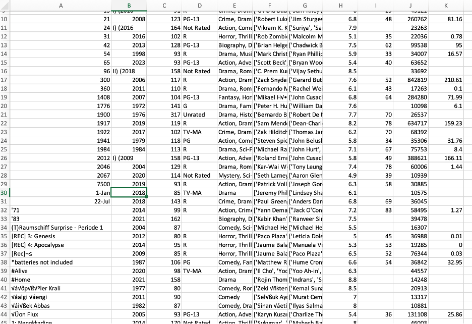
Rows beginning with special characters were deleted before the file was imported into SQL in Excel software. In PostgreSQL, a table was created for each of the two dataset files and the data imported from the .csv files. To join the datasets together, the following select statement was used:

SELECT m.title, mm.title as mm_title,  m.runtime, m.rating, m.metascore, m.votes, m.gross, mm.popularity, mm.revenue, mm.vote_average, mm.vote_count, m.stars,
CASE WHEN m.rating >= 7 THEN 'High'
           ELSE 'Low'
           END AS "rating-2",
case when position(',' in genre) = 0
            then substring(genre,1,length(genre))
            else substring(genre,1,(position(',' in genre) - 1))
            END as First_Genre,
split_part(replace(stars,'''',' '),',',1) as Star1,
split_part(replace(stars,'''',' '),',',2) as Star2
FROM public.movies AS m
inner join movies_metadata AS mm
          ON mm.title = m.title;

Logistical regression is a statistical tool used to show the relationship between the dependent variable and one or more independent variables and estimating the probabilities. The outcome of IMDb rating is numeric and ranges from 1-10, for this dataset. This variable will be put in two categories: “high” and “low” for the regression model. In the case with more than one independent variable are used, it is called multiple logistic regression.

This query included creating a row for the IMDb “rating” field and categorized the numeric data into a binary categorical value. This new variable was called “rating-2.” After encoding the dependent variable, the IMDb rating has two unique values, “high” and “low.” The “genre” variable contained multiple listed genres, but for analysis purposes, only the first one is retained. This query also includes a categorical field that chose the main genre and created a column called “first_genre.” The “stars” variable was in an array format and needed to be extracted in SQL. The first two main characters were preserved and placed into separate columns for analysis. These columns were labeled “star1” and “star2.”

Here is a screenshot of the exported combined dataset, also the full “data.csv” will be provided as an attachment with this analysis.

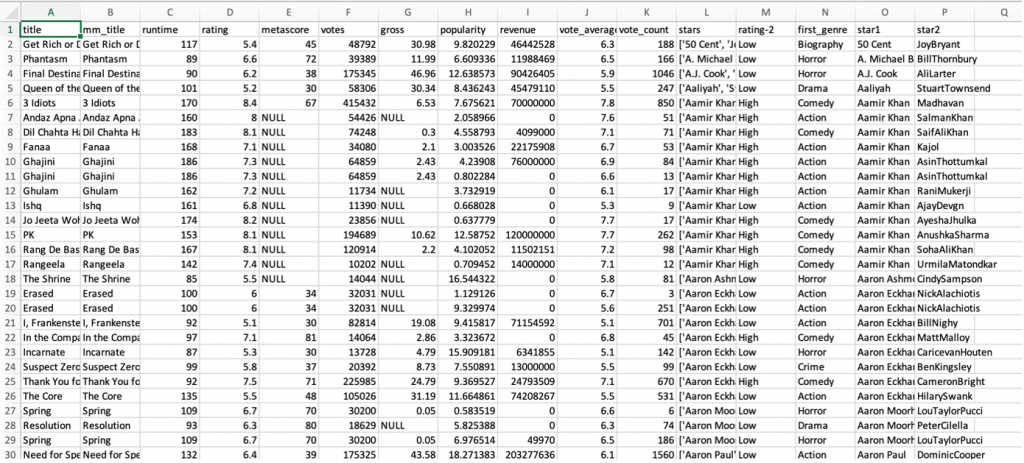
The exported .csv file from SQL needed two extra steps of cleaning special characters from the star fields. Find and replace tool was used to remove the brackets from the start variables.

After the csv file was exported from SQL, it was ready to be cleaned and preprocessed in Python. Python is the programming language used to run stats, analysis, models, and research for this task. Python comes with several packages that will be used for various parts of this analysis. Python is a powerful tool to use for logistic regression because statistical models for performing tests are found in several add-on libraries. For example, logit function has modeling tests and analysis built into the software with an easy install package line of script. Python makes it easy to run coefficient tests and statistics on datasets like the movie dataset. Jupyter Notebook is an online kernel to run Python using a web browser to import more packages, and libraries. Anaconda Navigator application runs Jupyter Notebook within a web browser and command prompt local sever. Anaconda Navigator has more than one thousand data sciences packages built in, which is easy to install and run. A MacBook pro laptop is used to install Anaconda application, run Python, export, and save datasets as well as save Jupyter Notebooks of Python code for future use.

Data preprocessing within Python consisted of handling and treating missing, duplicate, and outlier data. The feature selection which included deciding, based on statistics models, which variables had the most correlation with the dependent “rating” variable. Data exploration or EDA was performed to understand the distribution of variables, detect outliers, identify patterns, and find nulls. Feature selection in addition is performed to decide which variables to include in the model. Encoding categorical variables into numeric variables is performed on the dataset. Correlation statistics help mathematically identify which variables to include and exclude from the available numeric variables. These steps prepare the dataset for model building and evaluation. Following the preprocessing, the data will be split into two sets: one for training the regression model and one for testing the accuracy of the regression model.

The first step, see code below, was to import standard libraries and packages into Python, including Numpy, Pandas, Seaborn, Matplotlib, Pylab, Statsmodels, Scipy, and Sklearn.

import pandas as pd
import textwrap
import warnings

# Standard data science imports
import numpy as np
import pandas as pd
from pandas import Series, DataFrame 

# Visualization libraries
import seaborn as sns
import matplotlib.pyplot as plt 
%matplotlib inline # Statistics packages
import pylab
from pylab import rcParams
import statsmodels.api as sm
import statistics
from scipy import stats # Scikit-learn
import sklearn
from sklearn import preprocessing
from sklearn.linear_model import LinearRegression
from sklearn.model_selection import train_test_split
from sklearn import metrics
from sklearn.metrics import classification_report 

# Import chisquare from SciPy.stats
from scipy.stats import chisquare
from scipy.stats import chi2_contingency 
from sklearn.datasets import make_classification
from matplotlib import pyplot as plt
from sklearn.linear_model import LogisticRegression
from sklearn.model_selection import train_test_split
from sklearn.metrics import confusion_matrix
import pandas as pd

# Read the CSV file into a pandas DataFrame df = pd.read_csv('/Capstone/data.csv')

Import the .csv combined datasets file downloaded from SQL into Python and turn it into a dataframe called “df.”

To understand the data, Python has built-in features for obtaining an overview of information from the data, describing the data, and extracting statistical information. Statistical analysis helps in understanding parameters such as the mean, standard deviation, minimum and maximum values, and more. Python provides functions like .head(), .info(), and .describe() to accomplish this initial data analysis.

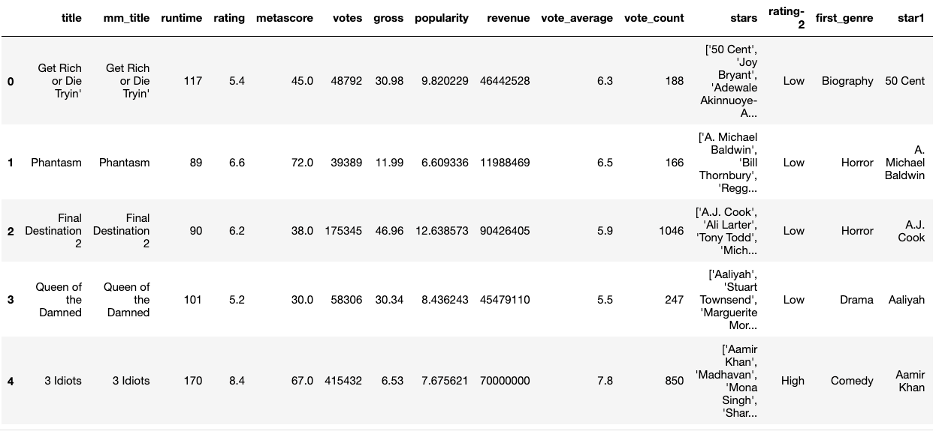
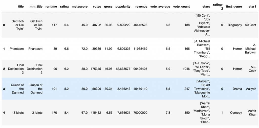
The head function is used to get an overview of the top rows of the dataset. To inspect the structure and contents of the dataset imported into Python.

df.head()

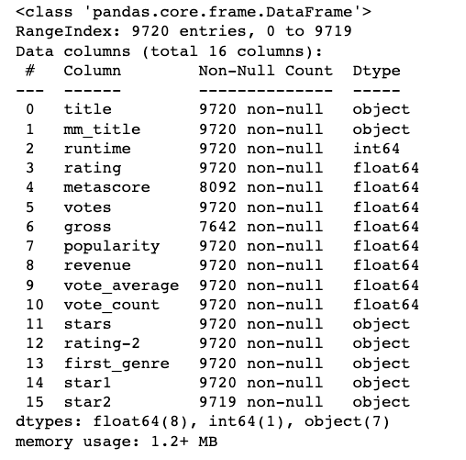
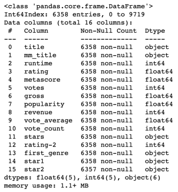
Provided by the panda’s library, the info function is used to view important analysis of the data frame, such as counts of non-null data and data types of variables. It’s a valuable tool for understanding the basic characters of the dataset. It is particularly useful during exploratory data analysis to quickly assess the distribution of your numeric variables and identify potential outliers or unusual patterns in the dataset.

df.info()

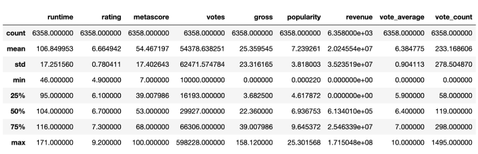
The summary statistics of the dataset overview is shown here in the describe function. Important information about each numerical variable is shown in a table format. Knowing the mean, or average value, of the column is helpful for remedying the null values. The standard deviation measures the amount of variation in the data. Minimum and maximum values help to remedy the outliers that show up in a variable.

#Print Dataframe
df.describe()

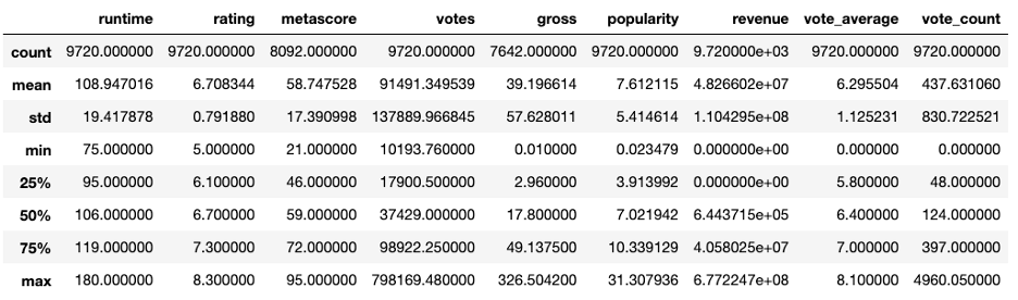
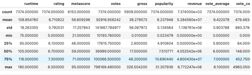
Duplicate entries can lead to overfitting the model. If machine learning models learn on repetitive information, it may perform poorly. That’s why it’s important to remove duplicates. The panda’s library offers drop_duplicates function to remove duplicate movies from the dataset. This takes the entries count from 9,720 to 7,374 in the dataset.

# Drop duplicates in 'title' while keeping the first occurrence
df = df.drop_duplicates(subset=['title'])

Identifying and handling missing data is accomplished by imputation or removing rows or columns. Pandas has a function .isnull to count the number of nulls in each variable. For this function it shows both categorical and numeric datatypes. However, running the describe function is key here, because the null values may show zero, but the describe function will show values of “0”. Here there are two columns that show null values that need to be treated, “metascore” and “gross.”

df.isnull().sum()

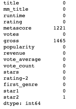
Learning from the description above, these two columns are numerical; hence, they can be utilized in the machine learning model. However, machine learning models cannot handle null values, so it is necessary to address these null values. To define and calculate the average value, or mean, of a variable, the Pandas library provides a built-in mean function. There are multiple ways to treat nulls, for this project the most common method used is imputation using the mean values was executed. Replacing the null values in the two variables with the mean as shown below.

# Calculate the mean of the numeric field
mean_value = df['gross'].mean()

# Fill missing values with the mean
df['gross'].fillna(mean_value, inplace=True)

# Calculate the mean of the numeric field
mean_value2 = df['metascore'].mean()

# Fill missing values with the mean
df['metascore'].fillna(mean_value, inplace=True)

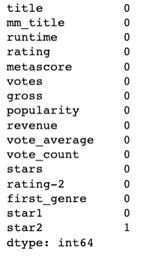
The isnull function was executed again and showed no null values existed after the imputation process.

After the data is cleaned, Exploratory Data Analysis (EDA) was performed on the provided variables in the dataset. EDA was performed to understand the distribution of variables and identify patterns. This provided insights into why ratings are given to movies. Outliers found in variables, such as ‘gross’ and ‘popularity,’ were identified and treated using the z_scores function from scipy.stats. During the EDA process, correlation graphs were generated to determine which variables had a higher correlation and should be included in the training dataset.

Univariate statistics is the analysis of a single variable at a time. To visualize the distribution of the single variables, histograms and boxplots are graphical tools used. The histogram for the binary categorized rating, “rating-2,” shows estimated 4,000 in the “low” category and 2,800 in the “high” category. Which is a good mix to train a ML model. The mean of the rating category is 6.664942.

plt.hist(df['rating-2'])
plt.show()

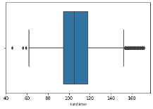
The “runtime” variable showed the presence of outliers. Treating these outliers, z-scores were computed and data points beyond a threshold of 3 standard deviations on either side of the mean were removed. The stats library calculated standard scores for this function. Below is the histogram of before and after the outliers have been removed using z-score calculations. The histogram showed the mean runtime for this dataset is 106.849953.

boxplot=sns.boxplot(x='runtime',data=df)

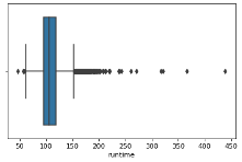
# Calculate the z-scores for the 'runtime' column
z_scores = stats.zscore(df['runtime'])

# Define a threshold to identify outliers
threshold = 3

# Identify the indices of outliers
outlier_indices = (z_scores > threshold)

# Remove the outliers from the DataFrame
df = df[~outlier_indices]

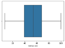
The “metascore” variable showed the presence of little to no outliers. The histogram showed the mean for metascore, for this dataset is 54.467197.

boxplot=sns.boxplot(x='metascore',data=df)

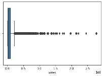
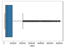
The “votes” variable showed the presence of outliers. To address these outliers, z-scores were computed, and data points beyond a threshold of 3 standard deviations on either side of the mean were removed. The stats library calculated standard scores for this function. Below is the histogram of before and after the outliers have been removed using z-score calculations. The histogram showed the mean votes for this dataset is 54,378.638251.

boxplot=sns.boxplot(x='votes',data=df)

# Calculate the z-scores for the 'votes' column
z_scores = stats.zscore(df['votes'])

# Define a threshold to identify outliers
threshold = 3

# Identify the indices of outliers
outlier_indices = (z_scores > threshold)

# Remove the outliers from the DataFrame
df = df[~outlier_indices]

boxplot=sns.boxplot(x='votes',data=df)

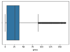
The “gross” variable showed the presence of outliers. To address these outliers, z-scores were computed, and data points beyond a threshold of 3 standard deviations on either side of the mean were removed. The stats library calculates standard scores for this function. Below is the histogram of before and after the outliers have been removed using z-score calculations. The histogram showed the mean gross for this dataset is 25.359545.

boxplot=sns.boxplot(x='gross',data=df)

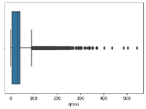
# Calculate the z-scores for the 'gross' column
z_scores = stats.zscore(df['gross'])

# Define a threshold to identify outliers
threshold = 3

# Identify the indices of outliers
outlier_indices = (z_scores > threshold)

 # Remove the outliers from the DataFrame
df = df[~outlier_indices]

boxplot=sns.boxplot(x='gross',data=df)

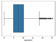
The “popularity” variable showed the presence of outliers. To address these outliers, z-scores were computed, and data points beyond a threshold of 3 standard deviations on either side of the mean were removed. The stats library calculates standard scores for this function. Below is the histogram of before and after the outliers have been removed using z-score calculations. The histogram showed the mean popularity for this dataset is 7.239261.

boxplot=sns.boxplot(x='popularity',data=df)

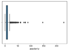
# Calculate the z-scores for the 'popularity' column
z_scores = stats.zscore(df['popularity'])

# Define a threshold to identify outliers
threshold = 3

# Identify the indices of outliers
outlier_indices = (z_scores > threshold)

# Remove the outliers from the DataFrame
df = df[~outlier_indices]

boxplot=sns.boxplot(x='popularity',data=df)

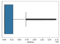
The “revenue” variable showed the presence of outliers. To address these outliers, z-scores were computed, and data points beyond a threshold of 3 standard deviations on either side of the mean were removed. The stats library calculates standard scores for this function. Below is the histogram of before and after the outliers have been removed using z-score calculations. The histogram showed the mean revenue for this dataset is 2.024554e+07.

boxplot=sns.boxplot(x='revenue',data=df)

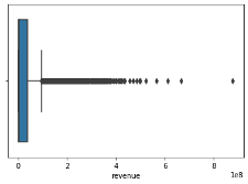
# Calculate the z-scores for the 'revenue' column
z_scores = stats.zscore(df['revenue'])

# Define a threshold to identify outliers
threshold = 3

# Identify the indices of outliers
outlier_indices = (z_scores > threshold)

# Remove the outliers from the DataFrame
df = df[~outlier_indices]

boxplot=sns.boxplot(x='revenue',data=df)

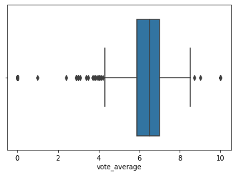
The histogram showed the mean for vote_average, for this dataset is 6.384775.

boxplot=sns.boxplot(x='vote_average',data=df)

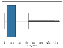
The “vote_count” variable showed the presence of outliers. To address these outliers, z-scores were computed, and data points beyond a threshold of 3 standard deviations on either side of the mean were removed. The stats library calculated standard scores for this function. Below is the histogram of before and after the outliers have been removed using z-score calculations. The histogram showed the mean vote_count for this dataset is 233.168606.

boxplot=sns.boxplot(x='vote_count',data=df)

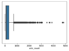
# Calculate the z-scores for the 'vote_count' column
z_scores = stats.zscore(df['vote_count'])

# Define a threshold to identify outliers
threshold = 3

 # Identify the indices of outliers
outlier_indices = (z_scores > threshold)

# Remove the outliers from the DataFrame
df = df[~outlier_indices]

boxplot=sns.boxplot(x='vote_count',data=df)

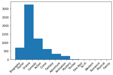
The genre variable was analyzed and showed which movies were popular among the genres. The “first_genre” variable extracted the first listed genre for the movie dataset. Drama genre was by far the most popular genre from this dataset.

# Extract the column for the histogram
values = df['first_genre']

#ignore warnings
warnings.filterwarnings('ignore')

# Create the histogram
plt.hist(values)

# Customize the x-axis labels (rotating them by 45 degrees)
plt.xticks(rotation=45)

# Display the plot
plt.tight_layout()

plt.show()

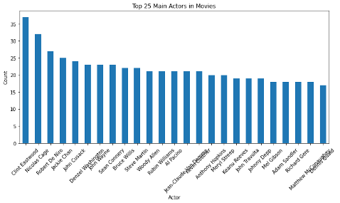
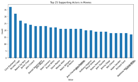
The “stars” variable, separated in SQL to extract the first star and second listed star into two columns. Both variables were analyzed to show which actors stared in popular movies in the cinema dataset.

# Group by actors and count how many times each actor appears
first_actor_counts = df['star1'].value_counts()

%matplotlib inline

# Select the top 25 actors based on their counts
top_25_actors = first_actor_counts.head(25)

# Plot the top 20 actors as a bar chart
plt.figure(figsize=(10, 6))

top_20_actors.plot(kind='bar')
plt.xlabel('Actor')
plt.ylabel('Count')
plt.title('Top 25 Main Actors in Movies')
plt.xticks(rotation=45)

# Display the chart
plt.tight_layout()
plt.show()

# Group by actors and count how many times each actor appears
second_actor_counts = df['star2'].value_counts()

# Select the top 25 actors based on their counts
top_25_actors = second_actor_counts.head(25)

# Plot the top 20 actors as a bar chart
plt.figure(figsize=(10, 6))

top_20_actors.plot(kind='bar')
plt.xlabel('Actor')
plt.ylabel('Count')
plt.title('Top 25 Supporting Actors in Movies')
plt.xticks(rotation=45)

# Display the chart
plt.tight_layout()
plt.show()

Before moving on to bivariate statistics a data describe function was executed again to get final statistics after the z-scores functions from the univariate statistics.

#Print Dataframe
df.describe()

Bivariate statistics is the analysis of two variables at a time. To visualize the distribution of the variable’s correlations, histograms, boxplots, and scatterplots are the graphical tools used for this analysis.

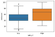
The below boxplot shows “rating-2” and “metascore” variables and how the correlate to each other. The metascore mean for the “low” category was about 47, while the metascore mean for the “high” category was much higher at about 67.

sns.boxplot(x='rating-2',y='metascore', data=df)
plt.show()

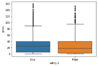
The below boxplot shows “rating-2” and “gross” variables and how the correlate to each other. The gross mean for the “low” category was about 25, while the gross mean for the “high” category was lower at about 18.

sns.boxplot(x='rating-2',y='gross', data=df)
plt.show()

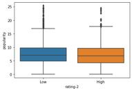
The below boxplot shows “rating-2” and “popularity” variables and how the correlate to each other. The popularity mean for the “low” category was about 7, while the popularity means for the “high” category very close at about 6.5.

sns.boxplot(x='rating-2',y='popularity', data=df)
plt.show()

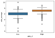
The below boxplot shows “rating-2” and “vote_average” variables and how the correlate to each other. The vote_average mean for the “low” category was about 6, while the vote_average mean for the “high” category next at about 7.

sns.boxplot(x='rating-2',y='vote_average', data=df)
plt.show()

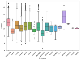
The below boxplot shows “runtime” and “first_genre” variables and how the correlate to each other. The average mean for runtime is 106 mins. The top three means based on genres are Western, Biography and Romance.

sns.boxplot(x='first_genre',y='runtime', data=df)

# Customize the x-axis labels (rotating them by 45 degrees)
plt.xticks(rotation=45)
plt.show()

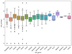
The below boxplot shows “vote_average” and “first_genre” variables and how the correlate to each other.The variable vote average has a mean of 6.38. The Western genre has a higher mean average, with Film-Noir and Biography genres averages higher.

sns.boxplot(x='first_genre',y='vote_average', data=df)

# Customize the x-axis labels (rotating them by 45 degrees)
plt.xticks(rotation=45)
plt.show()

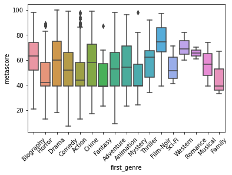
The below boxplot shows “metascore” and “first_genre” variables and how the correlate to each other.The mean metascore variable is 54.47. However, the mean metascores change based on the genre shown below. The highest mean score is Film-Noir cinemas, with Western and Romance genres closest next.

sns.boxplot(x='first_genre',y='metascore', data=df)

# Customize the x-axis labels (rotating them by 45 degrees)
plt.xticks(rotation=45)
plt.show()

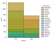
The below histogram shows count of rating-2 variable and how it correlates to genre. Action, comedy, and adventure are the top genres in the low category. Drama and action are the top genres for the high category.

sns.FacetGrid(df,hue = 'first_genre', height = 5).map(sns.histplot, 'rating-2').add_legend()

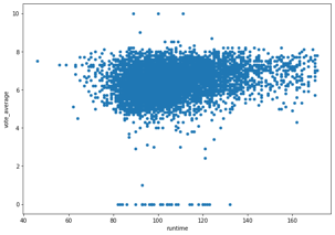
The below scatterplot shows the “vote_average” and “runtime” variables and how they correlate to each other. Our data summary indicates that the mean runtime is 106 minutes, and the mean “vote_average,” is 6.38. The scatterplot reveals that the intersection of these two mean variables is located right in the middle of the densest cluster of blue dots. From the graph there is a trend in lower scores for shorter runtimes.

df.plot.scatter(x='runtime', y='vote_average')

The scatterplot below illustrates the correlation between the ‘gross’ and ‘runtime’ variables. Our data summary indicates that the mean runtime is 106 minutes, and the average gross profit for the US and Canada, shown in millions, is 25. The scatterplot reveals that the intersection of these two mean variables is located right in the middle of the densest cluster of blue dots. However, there are two intriguing lines of dots at the lower end of the gross profit scale and around the 40 million gross profit mark. These two segments display a wide range of runtimes, spanning from 60 minutes to 170 minutes. Further research and analysis are needed to understand the factors contributing to these patterns.

df.plot.scatter(x='gross', y='runtime')

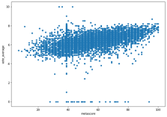
The scatterplot below illustrates the correlation between the ‘metascore’ and ‘vote_average’ variables. Our data summary indicates that the mean metascore is 54.47, and the average vote_average, is 6.38. The scatterplot reveals that the intersection of these two mean variables is located right in the middle of the densest cluster of blue dots. The graph suggests there is a slight increase of vote_average score based on the higher metascore. Further research and analysis are needed to understand the factors contributing to these patterns.

df.plot.scatter(x='metascore', y='vote_average')

Converting categorical variables into a numerical datatype, is an important step in machine learning to include non-numeric data for analysis. One-hot encoding and Label encoding are two techniques, built into the Python libraries to achieve this transformation. Categorical data types represent content categories, strings, or labels. There are nominal and ordinal categories data types. The target variable, IMDb rating is an ordinal categorical data type. There is a ranking order to this binary label data variable. For this project the .replace() function is used from the Pandas library to replace “yes” and “no” values in the rating variable. This encodes the ranking variable into a ‘int64’ from an ‘object’ data type.

# will replace "Yes" value in dataframe with 1
df = df.replace("High",1)

# will replace "No" value in dataframe with 0
df = df.replace("Low",0)

df.info()

df.head()

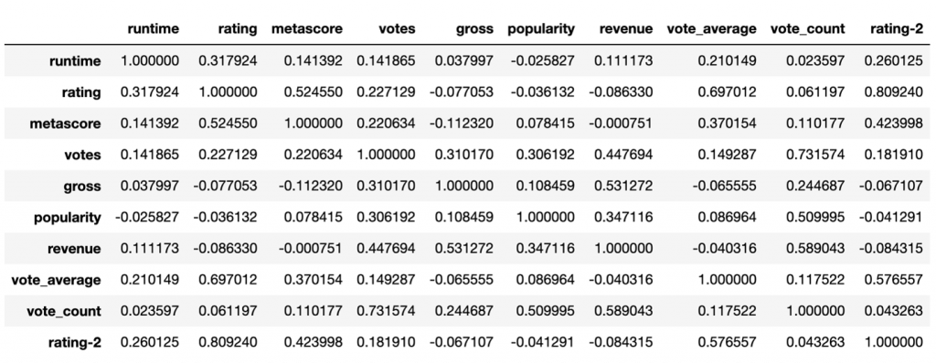
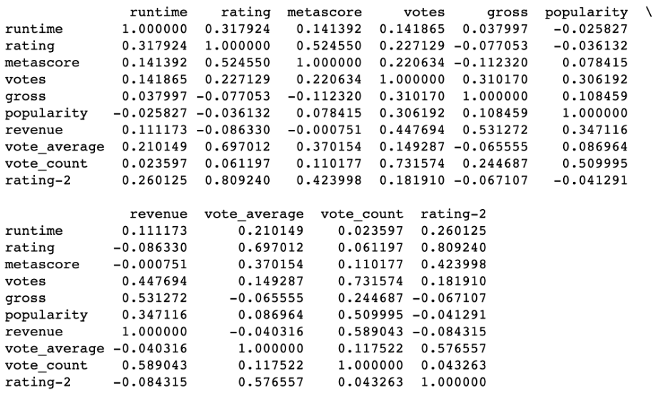
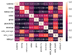
Deciding which predictors variables to include in the model is called feature selection. Correlation chart and heat map is used as the statistical technique for feature selection by the analyst. Variables that are highly correlated need to be included in the training model, and in contrast variables with lower scores are less correlated. For example, popularity, vote_count and votes variables are lower correlated to the ‘rating-2’ variable and therefore are excluded from the training regression model. In comparison, metascore, runtime, and vote_average variables are highly correlated to the rating column. These three variables are used to train the model to get the accuracy highest for this project.

df.corr()

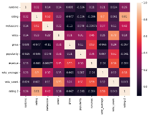
sns.heatmap(df.corr(), annot = True)
plt.rcParams['figure.figsize'] = (10,7)
plt.show()

corrMatrix = df.corr()
print (corrMatrix)

sns.heatmap(df.corr(), vmin=-1, vmax=1,
cmap= sns.diverging_palette(10, 400, as_cmap=True))

sns.heatmap(df.corr(), annot = True)
plt.rcParams['figure.figsize'] = (10,7)
plt.show()

The advantage of data extraction and preparation methods for logistic regression lies in the transformation of raw data into structured, encoded formats suitable for analysis. This process involves cleaning, filtering, and wrangling the data to prepare the variables for building machine learning models, such as regression. By using the cleaned data and selecting variables based on analytical statistics, the accuracy of model outcomes is enhanced. For example, the target variable chosen for this project was an ordinal categorical variable. To use the ranking variable as a binary numeric field, encoding variables made it possible to convert the ranking target variable into a prediction variable with two choices, “high” and “low.”

One disadvantage data extraction and preparation methods for logistic regression is the possibility of biases or errors in the dataset. When treating missing data and outliers, if not handled carefully this may negatively impact the model’s performance.

Analysis

The IMDb movie dataset was utilized to construct a logistic regression model for predicting a movie’s ranking based on several independent variables. The data analysis process involves multiple steps in data preparation. Logistic regression is a statistical method that entails training a machine learning model using independent variables to predict a binary dependent variable.

The original Internet Movie Database dataset used for creating this regression model included a ranking variable ranging from 1 to 10, indicating a movie’s success among fans. To build a machine learning regression model, this variable needed to be transformed into a binary format. With the assistance of variable encoding, this transformation was achieved, resulting in two choices of “high” and “low” for this variable.

During the Exploratory Data Analysis (EDA) process, the independent variables were visualized, providing valuable insights into which ones might be most suitable for predicting rankings. We could determine which combination of the multiple variables could be used to train the model with the highest accuracy only after conducting correlation statistics. This was a vital step in the data analysis process.

A training dataset is used to train the model, running congruously is a testing dataset to measure how accurate the ML model is performing. Data splitting makes this possible in Python. This technique divides the dataframe into two parts: training and testing. The user sets the percentage for each split, but common practice is 80/20 or 70/30.

X = df [['runtime', 'metascore', 'vote_average']]
y = df ['rating-2']

# Split the dataset into training and test dataset
X_train, X_test, y_train, y_test = train_test_split(X, y, random_state=1)

# Create a Logistic Regression Object, perform Logistic Regression
log_reg = LogisticRegression()
log_reg.fit(X_train, y_train)

LogisticRegression(C=1.0, class_weight=None, dual=False, fit_intercept=True    
           intercept_scaling=1, max_iter=100, multi_class='ovr', n_jobs=1,
          penalty='l2', random_state=None, solver='liblinear', tol=0.0001,
          verbose=0, warm_start=False)

When using logistic regression to build a machine learning model, the coefficients and intercept prove important as a key indicator of how the model is performing. This array of coefficients is connected to the feature variables of the model. Each coefficient represents the change in log-odds of the three target variables, in this case a binary classification. These were: 0.02446654, 0.03800871, 2.79872816. The last number in the array, -23.5575112, represents the intercept or log-odds of the target variable, ranking.

# Show to Coeficient and Intercept
print(log_reg.coef_)
print(log_reg.intercept_)

[[0.02446654 0.03800871 2.79872816]]
[-23.5575112]

To perform predictions for the logistic regression model on the test dataset ‘X_test’. These predictions were stored in the ‘y_pred’ variable. These steps measured the accuracy of the model for future predictions.

# Perform prediction using the test dataset
y_pred = log_reg.predict(X_test)

A confusion matrix is used to describe the evaluation of the performance of the regression model. The array shows the numbers for each of the following order: ‘true_negative’, ‘false_positive’, false_negative’, ‘true_positive.’ In the following array there were 885: true_negative, 112: false_positive, 117: false_negative, and 476: true_positive guesses on the testing dataset.

# Show the Confusion Matrix
confusion_matrix(y_test, y_pred)

array([[885, 112],
          [117, 476]])

Python libraries have built in evaluation methods and techniques to summarize how your model is performing. Accuracy, precision, and recall metrics are the main insights used for this evaluation. The accuracy metric measures the proportion of correctly predicted the right rating in the testing dataset. In this case, the model correctly predicted 85.6% of the time. The precision metric measures the amount of correctly predicted positive instances out of all the positive predictions in the model. In this case 81.0% of this model predicted as positive. The recall metric measures how many times the testing model correctly identified the sensitivity or true positive rate. In this case 80.3% recall rate. This regression model is preforming at a good rate of 80% accurate.

print("Accuracy:",metrics.accuracy_score(y_test, y_pred))
print("Precision:",metrics.precision_score(y_test, y_pred))
print("Recall:",metrics.recall_score(y_test, y_pred))

Accuracy: 0.8559748427672956
Precision: 0.8095238095238095
Recall: 0.8026981450252951

For logistic regression modeling, easier interpretations were achieved due to the analysis of each variable on a smaller dataset. This is possible due to the size of the dataset. For this capstone, the dataset analyzed consisted of ten variables to analyze. Larger and more complex datasets would make this process of analyzing and interpretability much longer and harder.

A disadvantage of data analysis in logistic regression was relying on the assumption of linearity for binary prediction outcomes. Identifying the independent variables that exhibit a linear correlation with the prediction variable proved to be time-consuming, requiring several iterations of combining independent variables to achieve the highest possible model accuracy.

Data Summary and Implications

This analysis began with the following research question and hypotheses:

Research Question What is the anticipated IMDb (Internet Movie Database) rating a movie can achieve by leveraging a set of explanatory variables extracted from a popular movie dataset?

Null hypothesis– The independent variables have no effect on the dependent variable, average IMDb movie rating of high or low from the Internet Movie Database.
Alternate Hypothesis– The independent variables influence the dependent variable, average IMDb movie rating of high or low from the Internet Movie Database.

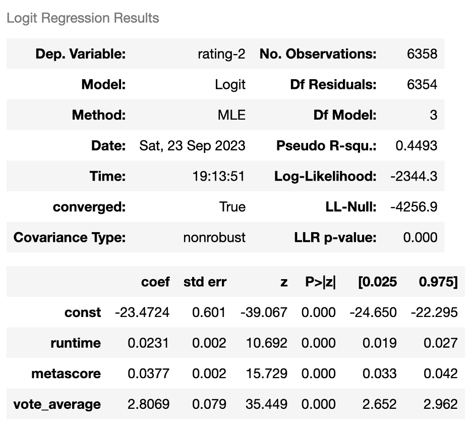
The final logistic regression prediction model, created in Python, had an accuracy of 0.8559748427672956. The logit regression results consisted of a summary of the coefficients, standard deviation error, z-statistic, p values, Pseudo R-squared, etc.

The number of observations of this model was 6,358. The dependent variable, which is the binary outcome variable used to predict the ranking of a movie’s success among fans. The independent variables, or feature variables, used was ‘runtime’, ‘metascore’, ‘vote_average.’ The pseudo r-squared score indicates a good fit model at 0.4493.

The bottom portion of the summary focuses on the scores of each independent variable has on the target variable. Coefficient represents the impact score of each feature variable has on the target variable. Those scores and variables are runtime: 0.0231, metascore: 0.0377, and vote_average: 2.8069.

The standard error statistic measured the uncertainty associated with the coefficient estimates. The smaller the errors are indicating more precise estimates. Those scores and variables are runtime: 0.002, metascore: 0.002, and vote_average: 0.079.

Z-statistic score is calculated by dividing the coefficient by standard error. This is the statistic to test the null hypothesis. The larger the z-statistic suggested a more significant impact of the variable. Those scores and variables are runtime: 10.692, metascore: 15.729, vote_average: 35.449.

P-value score needs to be less than 0.05. This score proves the variable is statistically significant in predicting the outcome. In this case the p-value for all the dependent variables is less than 0.05, indicating there is strong evidence to reject the null hypothesis, indicating the dependent variables do have an impact on the prediction ranking outcome.

Logistic regression model summary


 import statsmodels.api as sm
 Logit_model = sm.Logit(y, sm.add_constant(X)).fit()
 Logit_model.summary()

I’m delighted that the regression model achieved an accuracy of 86%. However, there were certain limitations that needed to be addressed to achieve this level of performance. The most significant limitation pertained to the availability of an adequate number of data points required to construct a statistically robust machine learning model. To accurately predict whether a new movie will receive a high or low rating, numerous factors come into play. The pandemic undeniably altered how fan’s view, rate, and watch movies. This project enabled the training of a machine learning model to forecast human behavior based on previous human opinions, thus allowing for predictions of future ratings. The larger movie dataset contained data that hadn’t been updated beyond 2017. If this data were updated to 2023, it’s possible that the model would have incorporated different variables or outcomes.

In terms of implementing this rating model system for predicting ratings in the cinema industry, it’s important to consider the historical context. The cinema rating duo, Siskel and Ebert, set the standard until 1999. Their ratings and opinions were grounded in their personal experiences with the movies they reviewed. Their success stemmed from their ability to provide contrasting perspectives and critiques based on their individual life experiences and opinions.

This machine learning prediction model is designed to replicate the tasks performed by human critics. It aims to demonstrate to the cinema industry which insights and indicators have the most significant impact on ratings.

There are several ways to advance this research project. A data analyst could construct a comparative linear regression model to predict a movie’s precise numeric rating, which is now achievable. Additionally, someone could conduct web scraping to acquire additional movie data, such as budgets, to gain deeper insights into the factors influencing a movie’s ratings. Further analysis could be performed to formulate a composite target variable, encompassing factors like votes cast, gross profit, budget, etc., instead of relying solely on an already established rating.

Sources:

Banik, Rounak. (2017). The Movies Dataset. Retrieved September 15, 2023 from https://www.kaggle.com/datasets/rounakbanik/the-movies-dataset

Devpura, Ashutosh. (August 2023). IMDb Top 10,000 Movies. Retrieved September 15, 2023 from https://www.kaggle.com/datasets/ashutoshdevpura/imdb-top-10000-movies-updated-august-2023

Sree. (2020, October 26). Predict Customer Churn in Python. Towards Data Science. https://towardsdatascience.com/predict-customer-churn-in-python-e8cd6d3aaa7

Li, Susan. (2017, September 28). Building A Logistic Regression in Python, Step by Step. Towards Data Science. https://towardsdatascience.com/building-a-logistic-regression-in-python-step-by-step-becd4d56c9c8

Datarmat. (2022, July 28). How to Perform Logistic Regression in Python(Step by Step). Data Science. https://www.datarmatics.com/data-science/how-to-perform-logistic-regression-in-pythonstep-by-step/

Stojiljkovic, Mirko. Logistic Regression in Python. Real Python. https://realpython.com/logistic-regression-python/

SalRite. (2018, December 15). Demystifying ‘Confusion Matrix’ Confusion. Towards Data Science. https://towardsdatascience.com/demystifying-confusion-matrix-confusion-9e82201592fd